
Table of Contents
Remote Sensing 2018 Weed Map Dataset
This page presents datasets for “WeedMap: A large-scale semantic weed mapping framework using aerial multispectral imaging and deep neural network for precision farming” published to MDPI Remote Sensing (link).
The following page details our sugar beet and weed datasets, including file naming conventions, sensor specifications, and tiled and orthomosaic data. To download the entire dataset (5.36GB), please head to this link.
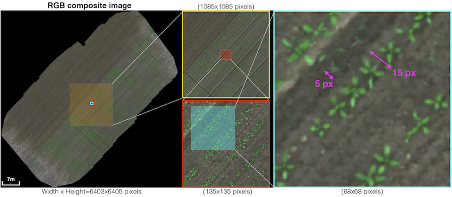
The picture below exemplifies one of the datasets used in this study. The left image shows the entire orthomosaic map, and the middle and right are subsets of each area at varying zoom levels. The yellow, red, and cyan boxes indicate different areas on the field, corresponding to cropped views. These details clearly evidence the large scale of the farm field and suggest the visual challenges in distinguishing between crops and weeds (limited number of pixels and similarities in appearance).
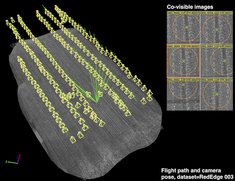
The figure below shows an example UAV trajectory covering a 1,300 square meter sugar beet field. Each yellow frustum indicates the position where an image was taken, and the green lines are rays between a 3D point and their co-visible multiple views. Qualitatively, it can be seen that the 2D feature points from the right subplots are properly extracted and matched for generating a precise orthomosaic map. A similar coverage-type flight path is used for our dataset acquisitions.
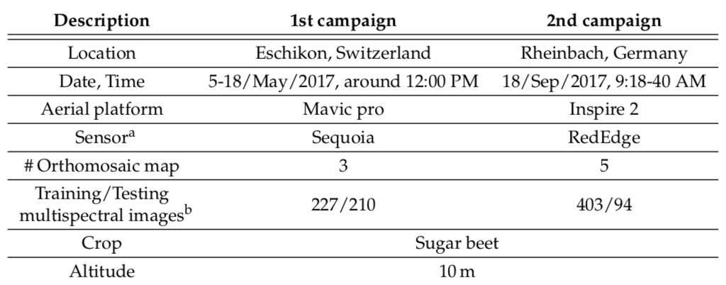
We collected datasets from sugar beet fields in Eschikon, Switzerland, and Rheinbach, Germany, with a time interval of five months (see the table below) using two commercial quadrotor UAV platforms carrying multispectral cameras, i.e., RedEdge-M and Sequoia from MicaSense.
Folder structure
The datasets consist of 129 directories and 18,746 image files, and this section explains their folder structure. We assume you downloaded the entire dataset (5.36GB).
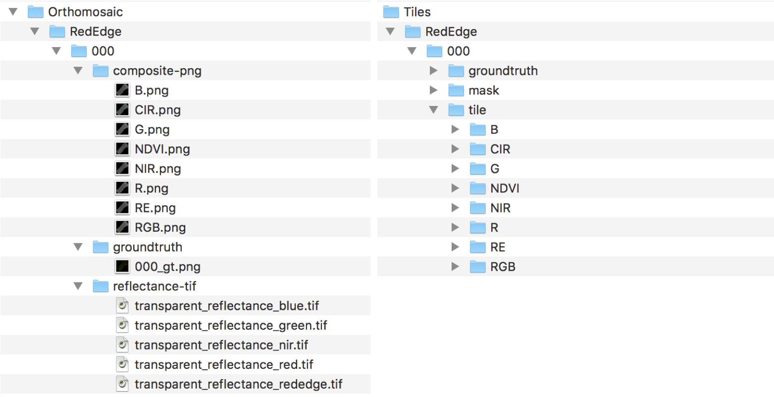 After the file extraction, you can find two folders named Orthomosaic and Tiles that contain orthomosaic maps and the corresponding tiles (portions of the region in an image with the same size as that of the input imag)e. We crop multiple tiles from an orthomosaic map by sliding a window over it until the entire map is covered.
Orthomosaic folder contains RedEdge and Sequoia subfolders that include 8 orthomosaic maps. Each of the subfolders indexed 000-007 and contains composite-png, groundtruth, reflectance-tif folders. Similar to Sequoia folder, there are 8 tiles and each contains groundtruth, mask, and tile folders.
Please find the overall folder structure from here.
File naming conventions
We indexed the datasets from 000 to 007 and believe most of file naming conventions are straightforward. For example, the groundtruth folder from Orthomosaic→ Rededge→000 contains orthomosaic image of dataset 000 (i.e., RedEdge dataset).
The same conventions applied to Tiles folder (e.g., 000-007 indicating dataset indices.), but groundtruth, mask, tile require more explanation.
The groundtruth folder contains manually labeled images and the original RGB (or CIR) images. The labelled images are in two formats; color and indexed images. The file convention of the former is “XXX_frameYYYY_GroundTruth_color.png” and “XXX_frameYYYY_GroundTruth_iMap.png” for the latter. XXX indicates dataset index (i.e., 000-007) and YYYY is the four-digit frame number starting from 0000 not 0001.
The color groundtruth images (i.e., XXX_frameYYYY_GroundTruth_color.png) represent each class in color; background=black, crop=green, weed=red whereas the index image (i.e., XXX_frameYYYY_GroundTruth_iMap.png) encodes these classes as numbers background=0, crop=1, weed=2, non-class=10000. The file format of color groundtruth image is 3 channel 8 bits PNG, 480×360 (width x height), and the index image is a grayscale of 16 bits.
The mask folder contains binary masks (white: valid, black: invalid) of the tile images. The file naming convention is “frameYYYY”, where YYYY indicates the frame number mentioned above.
The tile folders consist of 8 and 6 subfolders (RedEdge and Sequoia respectively). Each folder corresponds to a single channel and the file naming convention follows same as mask such that “frameYYYY” where YYYY indicates the frame number.
In case of questions, please feel to contact the Flourish team via e-mail: inkyu.sa@mavt.ethz.ch raghav.khanna@mavt.ethz.ch marija.popovic@mavt.ethz.ch.
Multispectral camera specifications
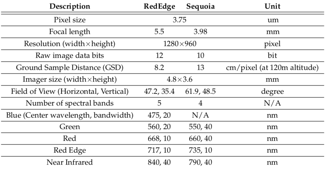
The table below elaborates the multispectral sensor specifications. More detailed product information can be found on the Micasense webpage (RedEdge-M and Sequoia).
Dataset summary
This section presents the summary of the datasets and downloading section for Orthomosaic and Tiles. If you want to download the entire dataset, use this link. We also provide a small portion of datasets for inspection purposes (~300MB). Please have a look at following sections: Orthomosaic small and Tile small.
The two data collection campaigns cover a total area of 16,554 square meters as shown in the table below. The two cameras we used can capture 5 and 4 raw image channels, and we compose them to obtain RGB and CIR images by stacking the R, G, B channels for an RGB image (RedEdge-M) and R, G, and NIR for a CIR image (Sequoia). We also extract the Normalized Difference Vegetation Index (NDVI). These processes result in 12 and 8 channels for the RedEdge-M and Sequoia camera, respectively. We treat each channel as an image, resulting in a total of 1.76 billion pixels composed of 1.39 billion training pixels and 367 million testing pixels (10,196 images). To our best knowledge, this is the largest publicly available dataset for a sugar beet field containing multispectral images and their pixel-level ground truth.
The input image size refers to the resolution of data received by our deep neural network (DNN). Since most CNNs downscale input data due to the difficulties associated with memory management in GPUs, we define the input image size to be the same as that of the input data. This way, we avoid the down-sizing operation, which significantly degrades classification performance by discarding crucial visual information for distinguishing crop and weeds.
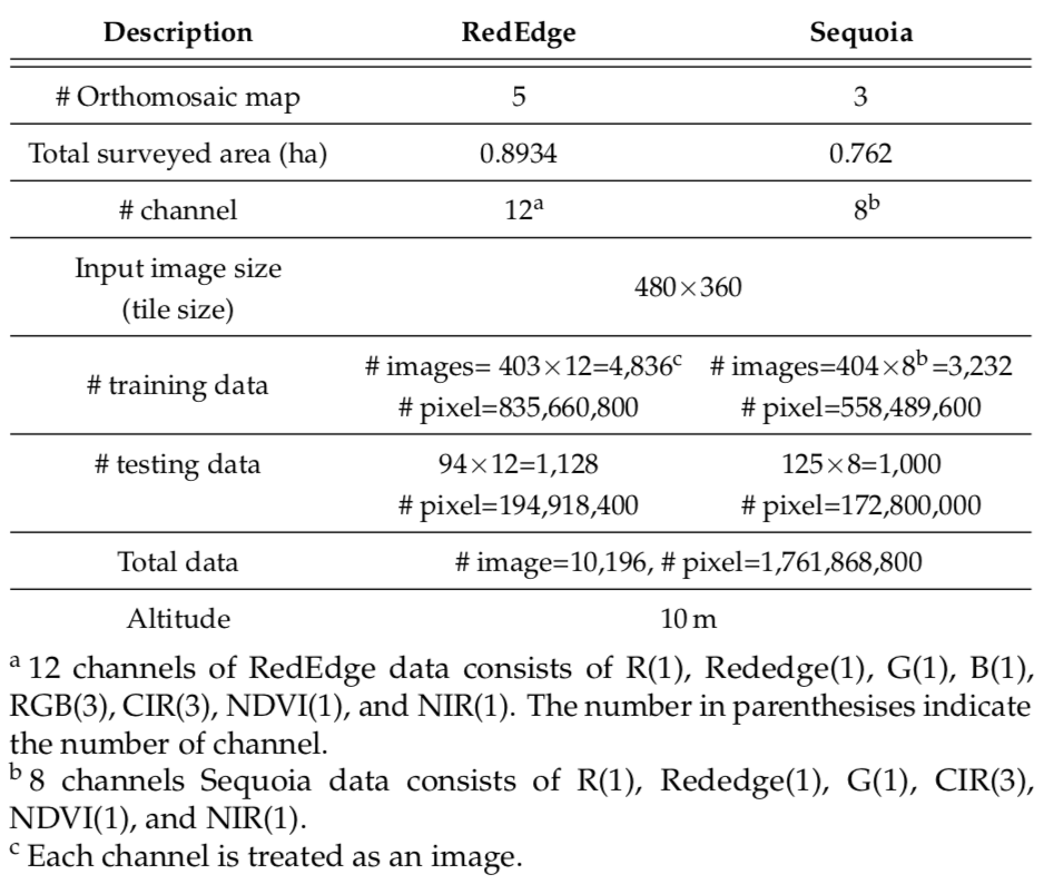
The table below presents further details regarding our datasets. The Ground Sample Distance (GSD) indicates the distance between two pixel centers when projecting them on the ground given a sensor, pixel size, image resolution, altitude, and camera focal length, as defined by its field of view (FoV). Given the camera specification and flight altitude, we achieved a GSD of around 1cm. This is in line with the sizes of crops (15-20 pixels) and weeds (5-10 pixels).

The number of effective tiles is the number of images actually containing any valid pixel values other than all black pixels. This occurs because orthomosaic maps are diagonally aligned such that the tiles from the most upper left or bottom right corners are entirely black images. The number of tiles in row/col indicates how many tiles (i.e., 480×360 images) are composed in a row and column, respectively. Padding information denotes the number of additional black pixels in rows and columns to match the size of the orthomosaic map with a given tile size. This information is used when generating a segmented orthomosaic map and its corresponding ground truth map from the tiles. We provide experimental MATLAB scripts that convert image tiles into an orthomosaic image and vice versa (see this section). The last property, attribute, shows whether the datasets were utilized for training or testing.
Orthomosaic
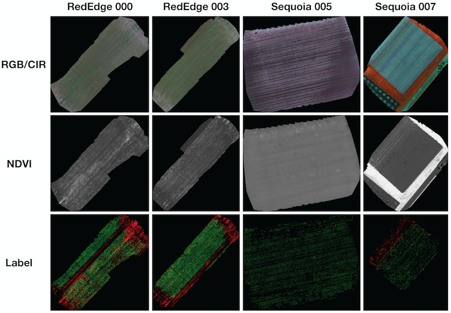
We provide 8 orthomosaic images and their corresponding labels. The figure below shows 4 samples of RGB/CIR, NDVI, and label for quality inspection purposes. If you want to proceed to the orthomosaic download section, please visit this section.
One can also try an interactive RGB and groundtruth comparison of one of the orthomosaic images (RedEdge-M, 000) by moving the center bar left or right for frame-by-frame comparisons.
RedEdge-M dataset 000, NDVI and RGB image comparison (try to move the center bar left or right for frame-by-frame comparisons).
Orthomosaic viewers
For better visualization, we also provide interactive zoom views of the high-resolution orthomosaic images.
(Ortho) RedEdge 5 channel multispectral images
(Ortho) Sequoia 4 channel multispectral images
Tiles
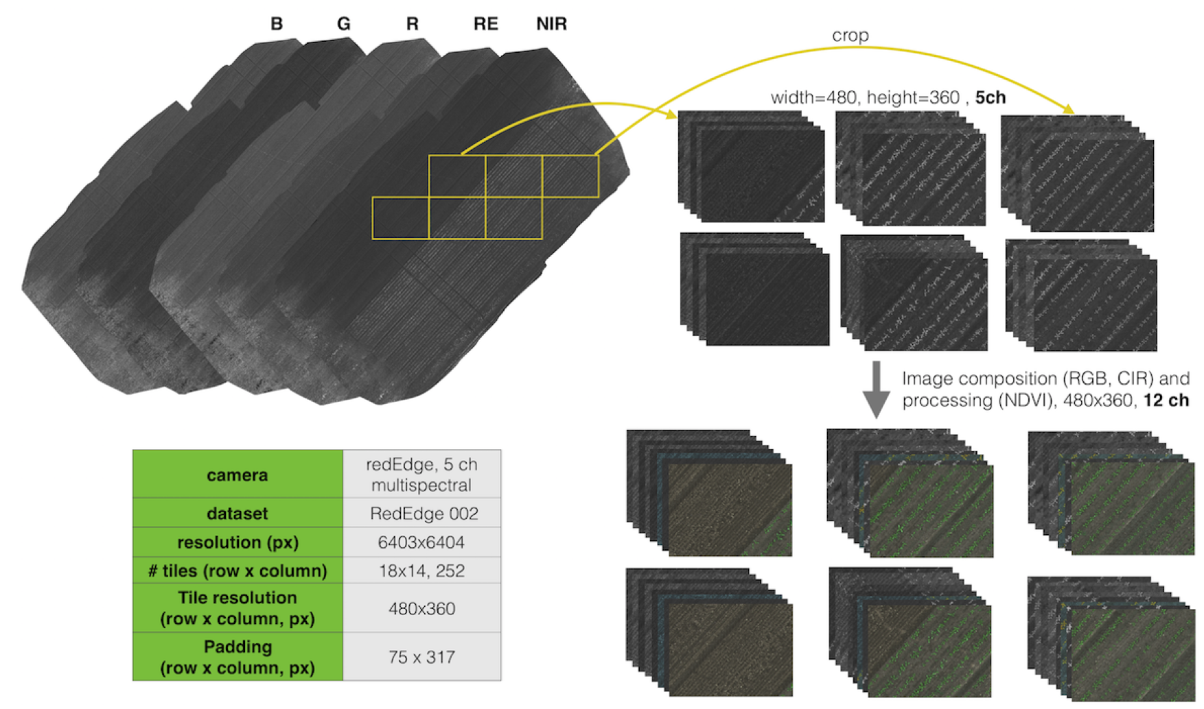
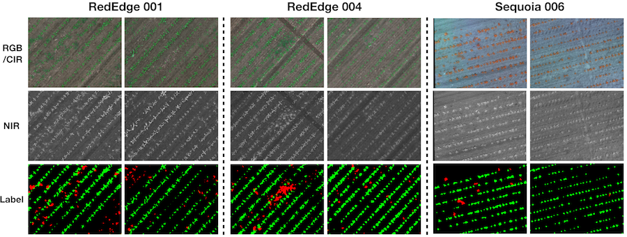
Similar to orthomosaic images, we provide 8 tiled images and their corresponding labels. The figure below illustrates the tiling preprocessing method for one of the datasets (RedEdge-M 002)
The figure below shows 4 samples of RGB/CIR, NDVI, and label for quality inspection purposes. If you want to proceed to the tile download section, please visit: this section.
One can also try an interactive RGB and groundtruth comparison of one of the tiled images (RedEdge-M, 000, frame number 0158) by sliding the center bar left or right.
RedEdge-M dataset 000, frame number 0158, NDVI and RGB image comparison (try to move the center bar left or right for frame-by-frame comparisons).
(Tile) RedEdge 5 channel multispectral images
(Tile) Sequoia 4 channel multispectral images
MATLAB Scripts for converting tile images into an orthomosaic
Under the scripts folder, there are two MATLAB scripts which convert an orthomosaic image → tiles (redEdge_from_ortho_to_tiles.m) and tiles → an orthomosaic image (redEdge_from_tile_to_ortho_ground_truth.m). These scripts tested on Mac High-Sierra (10.13.5), MATLAB 2017b, but are still experimental in order to demonstrate how to use the padding information when converting from tiles to an orthomosaic image.
Citation
If our study helps your works in an academic/research context, please cite the following publication: I. Sa, M. Popovic, R. Khanna, Z. Chen, P. Lottes, F. Liebisch, J. Nieto, C. Stachniss, A. Walter, and R. Siegwart , “WeedMap: A large-scale semantic weed mapping framework using aerial multispectral imaging and deep neural network for precision farming”, 2018, MDPI, Remote Sensing link
@ARTICLE{weedMap-2018,
author={I. Sa, M. Popovic, R. Khanna, Z. Chen, P. Lottes, F. Liebisch, J. Nieto, C. Stachniss, A. Walter, and R. Siegwart},
journal={MDPI Remote Sensing},
title={WeedMap: A large-scale semantic weed mapping framework using aerial multispectral imaging and deep neural network for precision farming},
year={2018},
volume={10},
number={9},
doi={doi: 10.3390/rs10091423},
month={Aug}}