Table of Contents
Tilting Laser
Platform Description
The platform was built to record point cloud datasets with some supporting data. A rotating support is connected via a 1:1 belt to a Maxon motor RE 25 (24 V) with planetary gear reduction (411:1). An encoder (HEDL 5540) is on the primary shaft of the motor with a precision of 500 counts per tick. After some preliminary tests, it was realized that the gear and the belt play introduce an uncertainty of approximately 5 degrees on the rotating support orientation. A second encoder (AEDA-3300TCH) with a precision of 48000 counts per tick was added on the rotating support axis (end effector) to cope with the uncertainty. Precise position homing is achieved using the third channel of the AEDA-3300TC. Both encoders are used in a dual regulation loop ensured by a Maxon Motor EPOS controller. This rotating support can be reconfigured to hold separately 4 sensors:
- Hokuyo UTM-30LX Data Sheet
- Hokuyo URG-04LX
- SICK LMS1xx Data Sheet
- Kinect
Sensor supporting data are:
- Xsens MTi-G (IMU, compass and GPS fixed on the frame) Data Sheet
- Point Grey Flea 2 (color camera mounted on rotating axis) Data Sheet
Note: For the datasets Laser Registration, only a Hokuyo with the Xsens were used.
Recording Methodology
The recording process is quite manual, so about 2-3h are required to record a dataset of 35 3D scans. The scanner is moved from a location to another one by an operator. Extra precautions are taken to ensure that the scanner stays in place while scanning (usually 20 sec) and while the ground truth position is measured (about 2 min). On a hard floor, robber foot are used whereas on soft ground, spikes are used. The inertia of the platform also ensure a good stability while recording a scan.
Global Positioning
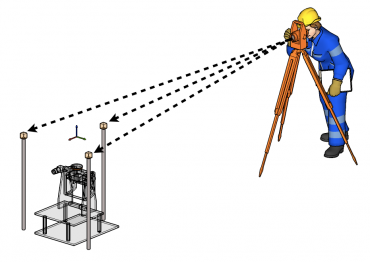
The main characteristics of the scanner is the possibility to record its position in a global referential frame with the help of an external sensor. To achieve a global positioning method that is independent of the registration algorithms, we used the TS15, a theodolite from Leica Geosystems. Theodolites are used for road and building surveys, and the system used here ensures 1-mm precision over 1 kilometer distance when combined with specialized prims.
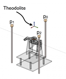
The Leica theodolite measures only one location at a time, i.e. one single point on a given object (here the scanner), which implies that 3 measurements are necessary to retrieve the complete pose of that object (translation and orientation). A specialized reflective prism (Mini 360) is mounted on a pole and thus, the prism can be secured at 3 different location on the scanner, namely  ,
,  and
and  (see figure below).
The pole is higher than the scanner to enhance visibility of the theodolite.
The reconstruction of the pose (6 DoF) in a global frame is computed as follow.
The translation components are selected to be at the center of mass of the 3 points.
By defining the vectors  and
and  , we can express the rotation components as:

Then, the transformation matrix becomes:

The first pose of the scanner recorded with this method is used as an offset to allow this first scanner pose to be taken as the origin of the dataset. In some cases, a complete dataset cannot be recorded within a single line of sight of the theodolite. In those situations, we first moved the theodilite while letting the scanner at an already recorded pose. Then, we can use the scanner pose as a beacon to relocalize the theodolite at its new position and we continue to move the scanner.
Frames and Calibration
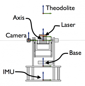 Multiple frames are used in the system:
Base (B): base of the scannerIMU (I): origin of the Xsens as defined in there documentationAxis (A): rotation point controlled by the motorCamera (C): optical center of a pin-point camera modelLaser (L): origin of the sensor producing pointsTheodolite (T): measured by an external sensor to determine the ground truth pose of the scanner. See the section Global Positioning for more information.
All the transformation are given the notation  , which can be read as:
the transformation
  that can express a point, originally in
  coordinate frame, in
  coordinate frame.
Translation vector
  is represented as [tx, ty, tz] and the rotation vector
  is represented as a quaternion [qx, qy, qz, qw].
| Transformation | Translation | Quaternion |
|---|---|---|
 | [0, 0, 0.22] | [0, 0, 0, 1] |
Mechanically measured. The offset between the homing position and the position with the rotating frame parallel to the Base is directly added in the low level controller (EPOS). This offset has been measured using 2 lasers fixed on the Axis and on the Base projecting points on a wall, 8 meters away. The angular position changes during one scan and it is measured using an encoder with 48000 counts per tick |
||
 | [0, 0, -0.085] | [0, 0, 0, 1] |
| Mechanically measured. | ||
 | [0.011, -0.009, 0.638] | [0.0026, 0.0100, -0.0063, -0.9999] |
| Adjusted with a global optimization method. See section Theodolite Calibration | ||
 (UTM-30LX) (UTM-30LX) | [0, 0, 0.04] | [0, 0, 0, 1] |
| Mechanically measured. The center of the laser has been determined using Hokuyo specifications. | ||
 (URG-04LX) (URG-04LX) | [TBD] | [TBD] |
 (LMS1xx) (LMS1xx) | [TBD] | [TBD] |
 (Kinect) (Kinect) | [TBD] | [TBD] |
 | [TBD] | [TBD] |
If you prefer to use a 4 by 4 transformation matrix instead of translation vector and quaternion, here is how to do the conversion:

Theodolite Calibration
Our global pose is given with respect to the frame Theodolite while the point clouds are constructed in the reference frame Base.
To compute the fixed correction between those two frames, we selected a controlled environment (i.e., a corridor) that provide 6 DoF constrained and we scanned it several times.
Then, we computed the global pose of Base as if the transformation  would equal the identity matrix.
In post-processing, we computed the alignment error
  using an Iterative Closest Point Algorithm (Pomerleau et al. IROS 2011). A global minimization algorithm reduces that error, which gives us the transformation between those frames:

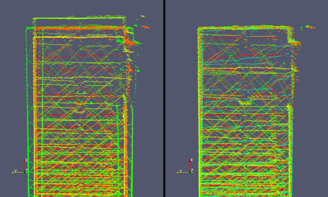
The figure below presents the impact of the calibration procedure. The color represents 3D scans of the same corridor with different poses. The calibration environment was selected to be highly constrained and scans were manually adjusted. This controlled protocol ensures that the ICP converges to the global minimum.
Ground Truth Evaluation
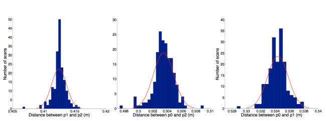
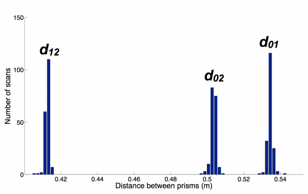
We evaluated the precision of this positioning method over 181 scanner positions.
We moved the scanner over different types of ground.
For every pose, we measured the position of  ,
,  and
and  to evaluate the stability of distances between the 3 prisms (
 ,
,  and
and  ).
The mean and standard deviation (std) for every segment are presented in the following table:
| Mean | Std | |
|---|---|---|
 | 412.5 mm | 1.2 mm |
 | 503.5 mm | 1.4 mm |
 | 534.4 mm | 1.4 mm |
The figure below depicts the estimated normal distributions against the sampled distributions, which show that the noise is Gaussian.
The std can mainly be due to manipulation errors and can exceed the manufacturer specification of 1 mm over kilometer range. Reasons that can explain such discrepancy may be that the scanner had moved while the prism is installed to another position, the pole supporting the prism had vibrated, the person moving the prism had confused the sequence of position, etc. Several systems were set in place to minimize the impact of those events. The weight of the scanner has been increased to augment its inertia. First, the feet of the scanner can either be 5-cm spikes for soft ground or rubber disks for hard ground. Second, a software monitors the theodolite readings and rejects every sequence of 3 points if the distance variations is larger than 3.5 mm. Moreover, since the mean distance between the prism's positions is significantly different (see figure below), the expected sequence of measurements can be validated by removing the chances of confusing the order of 2 positions while changing the prism position.
All those elements insure that a high-precision measurement of the scanner pose can be made in a multitude of environments. Sometimes, a sequence of scanner poses cannot be measured from a single theodolite position. For example, this happens when the scanner needs to turn a corner. To overcome this limitation, we use the scanner as a marker to relocalize the theodolite in its new pose. This slightly increases the localization error due to cumulation, but the precision is still in the range of millimeters.
How to Move Point Clouds from a Base Frame to a Global Frame?
Point clouds expressed in local frame (i.e.: with the origin located in the middle of the scanner) are named Hokuyo_<i>.csv, where <i> is an integer corresponding to the  of the scanner (see Hokuyo_<i>.csv for more details on that file).
Once you select a file, you can construct a matrix containing the column x, y, and z of the file as follow:
 , where
  is the number of lines in the file.
The poseId <i> of the file Hokuyo_<i>.csv also corresponds to a row in the file pose_scanner_leica.csv (see pose_scanner_leica.csv for more details on that file). A transformation matrix can be deserialized using the columns T00 to T33 as follow:

Finally, the point cloud  can be transformed in global coordinates like this:

Note that for all datasets, the origin of the global coordinate frame is located at the center of the scanner when the first scan was taken. Therefore, in the file pose_scanner_leica.csv, the transformation corresponding to poseId 0 is always identity.
File Formats
The section provides information on the content of each file produced by the tilting scanner. All file formats used, except rosbags, can be open in a text editor.
For all coma separated values (CSV) files, a table with the header and an example of the 2 first lines are explained.
Files in Base Frame (CSV)
Hokuyo_<i>.csv
In the file name, <i> is replaced by the poseId of the scanner, which starts at zero and is incremented every time the scanner changes position.
There is a line per point.
The header has the following elements:
- Time_in_sec: timestamps are recorded for each 2D scan produced by the Hokuyo and then uniformly distributed to all points of the 2D scan to reconstruct a timestamp per point (second)
- x, y, z: coordinates of laser point expressed in local frame (meter)
- Intensities: intensity returned on each beam. If -1, values weren't recorded
- 2DscanId: start at 0 and is incremented every time as 2D scan is taken
- PointId: start at 0 and is incremented for every point. The value reset at zero for every 2D scan.
| Time_in_sec | x | y | z | Intensities | 2DscanId | PointId |
|---|---|---|---|---|---|---|
| 1326899528.52450228 | -2.83598852 | -4.26281786 | 2.55458331 | -1.00000000 | 0 | 0 |
| 1326899528.52451968 | -2.83664942 | -4.30161667 | 2.55511546 | -1.00000000 | 0 | 1 |
| … | … | … | … | … | … | … |
xsens_compass_<i>.csv
In the file name, <i> is replaced by the poseId of the scanner, which starts at zero and is incremented every time the scanner changes position.
There is a line per reading and those readings span over the recording time of one 3D scan.
The header has the following elements:
- Time_in_sec: timestamps are recorded for each reading (second)
- Mx, My, Mz: vector pointing in the direction of the magnetic North and expressed in the local frame. The vectors aren't normalized
| Time_in_sec | Mx | My | Mz |
|---|---|---|---|
| 1326899528.36866832 | 0.07830320 | 0.55835843 | -0.50733519 |
| 1326899528.42052960 | 0.07748424 | 0.55837405 | -0.50801909 |
| … | … | … | … |
xsens_gps_<i>.csv
In the file name, <i> is replaced by the poseId of the scanner which start at zero and is incremented every time the scanner changes position.
There is a line per reading and those readings span over the recording time of one 3D scan.
The header has the following elements:
- Time_in_sec: timestamps are recorded for each reading (second)
- Latitude: GPS latitude (degree)
- Longitude: GPS longitude (degree)
- Altitude: altitude over sea level (meter)
- Nbsat_max_qualitysignal: number of satellites with the maximum quality signal
- Nbsat_locked: number of satellites detected
- valid_data: 1 = gps position could be evaluated, 0 = coordinates are invalid
| Time_in_sec | Latitude | Longitude | Altitude | Nbsat_max_qualitysignal | Nbsat_locked | valid_data |
|---|---|---|---|---|---|---|
| 1326899528.36866212 | 47.37632751 | 8.55028820 | 499.53897095 | 1 | 5 | 1 |
| 1326899528.42052341 | 47.37632751 | 8.55029106 | 498.87530518 | 1 | 5 | 1 |
| … | … | … | … | … | … | … |
xsens_gravity_<i>.csv
In the file name, <i> is replaced by the poseId of the scanner, which starts at zero and is incremented every time the scanner changes position.
There is a line per reading and those readings span over the recording time of one 3D scan.
The header has the following elements:
- Time_in_sec: timestamps are recorded for each reading (second)
- gx, gy, gz: Orientation of the gravity vector in local frame. It is normalized to one.
| Time_in_sec | gx | gy | gz |
|---|---|---|---|
| 1326899528.36866999 | -0.01402350 | -0.01421853 | -0.99980057 |
| 1326899528.42053127 | -0.01321996 | -0.01386344 | -0.99981650 |
| … | … | … | … |
Files in Global Frame (CSV)
PointCloud<i>.csv
In the file name, <i> is replaced by the poseId of the scanner, which starts at zero and is incremented every time the scanner changes position.
There is a line per point. It is the equivalent of Hokuyo_<i>.csv but the points are expressed in global coordinates based on pose_scanner_leica.csv.
To compute the transformation yourself read: How to move point clouds from a local frame to a global frame?.
The header has the following elements:
- Time_in_sec: timestamps are recorded for each 2D scan produced by the Hokuyo and then uniformly distributed to all points of the 2D scan to reconstruct a timestamps per point (second)
- x, y, z: coordinates of laser point expressed in global frame (meter)
- Intensities: intensity returned on each beam. If -1, values weren't recorded
- 2DscanId: start at 0 and is incremented every time a 2D scan is taken
- Points: start at 0 and is incremented for every point. The value reset at zero for every 2D scan.
| Time_in_sec | x | y | z | Intensities | 2DscanId | Points |
|---|---|---|---|---|---|---|
| 1323442000.736520 | -2.242188 | -2.962129 | 2.076716 | -1.000000 | 0 | 0 |
| 1323442000.736537 | -2.204924 | -2.938987 | 2.046712 | -1.000000 | 0 | 1 |
| … | … | … | … | … | … | … |
pose_scanner_leica.csv
This file content the pose of the scanner considered as “ground truth” using an external sensor (a theodolite from Leica).
To compute the transformation yourself, read:
- poseId: start at 0 and is incremented every time the scanner is moved to another location
- timestamp: not synchronized with other timestamps. The field poseId should be used to know which position goes with which files
- T00 to T33: Element of the transformation matrix. See How to move point clouds from a local frame to a global frame? for more information.
The header has the following elements:
| poseId | timestamp | T00 | T01 | T02 | T03 | T10 | T11 | T12 | T13 | T20 | T21 | T22 | T23 | T30 | T31 | T32 | T33 |
|---|---|---|---|---|---|---|---|---|---|---|---|---|---|---|---|---|---|
| 0 | 1323405881.0 | 1.0 | 0.0 | 0.0 | -0.0 | -0.0 | 1.0 | 0.0 | -0.0 | -0.0 | 0.0 | 1.0 | -0.0 | 0.0 | 0.0 | 0.0 | 1.0 |
| 1 | 1323406019.0 | 0.98 | -0.14 | 0.009 | 0.49 | 0.14 | 0.98 | -0.02 | 0.05 | -0.005 | 0.02 | 0.99 | 0.014 | 0.0 | 0.0 | 0.0 | 1.0 |
| … | … | … | … | … | … | … | … | … | … | … | … | … | … | 0.0 | 0.0 | 0.0 | 1.0 |
Note that the actual file has 6 digit precision, which were reduced in the table so it can fit in this web page.
xsens_Compass_mean.csv
This file has a line per scanner pose, resuming all xsens_compass_<i>.csv files in one. A mean over the columns of each file has been calculated to extract a single value per poseId. Also, vectors have been rotated to be expressed in global frame using the transformation in pose_scanner_leica.csv.
The header has the following elements:
- poseId: start at 0 and is incremented every time the scanner is moved to an other location
- Timestamp: timestamps are recorded for each reading (second). It is not synchronized and the field poseId should be preferred to associate other files.
- Mx, My, Mz: mean coordinates of the vector pointing in the direction of the magnetic North and expressed in the local frame. The vectors aren't normalized.
| poseId | Timestamp | Mx | My | Mz |
|---|---|---|---|---|
| 0 | 1323442009.456403 | -0.544021 | 0.019491 | -0.874596 |
| 1 | 1323442147.008762 | -0.557742 | -0.006950 | -0.874140 |
| … | … | … | … | … |
xsens_Gps_mean.csv
This file has a line per scanner pose, resuming all xsens_gps_<i>.csv files in one. A mean over the columns of each file has been calculated to extract a single value per poseId while only keeping values with the field valid_data set to 1.
The header has the following elements:
- poseId: start at 0 and is incremented every time the scanner is moved to another location
- Timestamp: timestamps are recorded for each reading (second). It is not synchronized and the field poseId should be preferred to associate other files.
- Latitude: GPS latitude (degree)
- Longitude: GPS longitude (degree)
- Altitude: altitude over sea level (meter)
- Nbsat: number of satellites detected
- valid_data: 1 = gps position could be evaluated, 0 = coordinates are invalid
| poseId | Timestamp | Latitude | Longitude | Altitude | Nbsat | valid_data |
|---|---|---|---|---|---|---|
| 0 | 1323446931.553646 | 47.375446 | 8.550164 | 491.810153 | 2 | 1 |
| 1 | 1323447023.102194 | 47.375321 | 8.550299 | 501.806665 | 6 | 1 |
| … | … | … | … | … | … | … |
xsens_Gravity_mean.csv
This file has a line per scanner pose, resuming all xsens_gravity_<i>.csv files in one. A mean over the columns of each file has been calculated to extract a single value per poseId.
The header has the following elements:
- poseId: start at 0 and is incremented every time the scanner is moved to another location
- Timestamp: timestamps are recorded for each reading (second). It is not synchronized and the field poseId should be preferred to associate other files.
- gx, gy, gz: orientation of the gravity vector in local frame. It is normalized to one.
| poseId | Timestamp | gx | gy | gz |
|---|---|---|---|---|
| 0 | 1323442009.456405 | 0.093112 | 0.032780 | -0.995096 |
| 1 | 1323442147.008763 | 0.091654 | 0.030511 | -0.995320 |
| … | … | … | … | … |
Visualization Files (VTK)
File type chosen for visualization is VTK legacy in ASCII format. We suggest to use Paraview to view the files because it can be freely downloaded for Windows, Mac and Ubuntu user and it's supported by Kitware. All screenshots of this page were realized using this software. You can download it here: http://www.paraview.org/
The files provided are:
- PointCloud<i>.vtk, where <i> is the 3D scan pose ID.
- path.vtk: Path of the scanner represented as a line on which each vertex contains information represented as scalar (3D pose ID, timestamp, High, Latitude, Longitude, Number of satellites) or vector (x-axis, y-axis and z-axis of the scanner, gravity, magnetic North) all represented in global frame.
- globalMap.vtk: single file in which all point clouds have been preprocessed (see section Suggested Preprocessing) and then concatenated into one global map with approximately 500 000 points.
How to visualize data using Paraview
Coming soon
Raw Recording (ROS Bags)
This type of data can be useful if you want to do some preprocessing on the 2D scans directly.
We used ROS (www.ros.org) as middleware so the raw recordings can be downloaded and playback using rosbag. One rosbag has been recored per 3D scan.
For more information on how to used this format see: www.ros.org/wiki/rosbag
Note: we used an obsolete version of the Xsens driver with custom ROS messages. Those definitions can be found here

